Series impedance vs input impedance

September 05, 2025

Introduction

When doing acoustic measurements, people often get confused by the abundance of words with 'impedance' in them. Each one has a different meaning. But what are these and what do they mean? When postprocessing a measurement, we have the choice from either series impedance or input impedance:

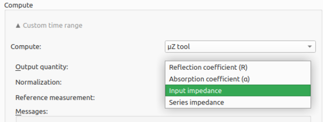
Screenshot of ACME, showing the µZ tool postprocessing output options

Here we are going to explain the details about these impedances.

µZ 4 microphone measurement method

When performing a measurement using the µZ system, a typical configuration is schematically shown below:

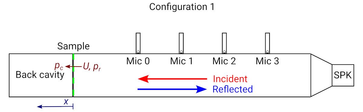
Impedance tube configured with a sample and back cavity

In this figure, the acoustic pressure ¹ at the tube side of the sample, is denoted by $p_r$, the acoustic pressure just at the other side. Note that the coordinate system $x$ has its origin at the sample, and is positive in the direction away from the speaker. The volume flow through the sample is defined as $U$. It is positive in $x$-direction.

The blue arrow indicates the incident wave and the red arrow indicate the reflected wave that we are able to measure. From these, the input impedance at the sample can be determined.

• The input impedance is the acoustic impedance at the sample as felt by the air in front of the sample, so it is defined as $Z_i =p_r/U$.
• The series impedance of the sample is defined as $Z_s = \left(p_r-p_c\right)/U$.

The acoustics of a sample can be defined by its series impedance when the sample is small with respect to the wavelength. In that case the volume flow $U$ is the same on both sides of the sample. This is a property of the sample itself alone², not of the system. If the series impedance is purely real, the direct electrical equivalent is a resistor.

The input impedance is not only dependent on the sample, but also on what is on the other side of the sample. In the figure above this is a back cavity with a certain dimension.

Another possibility is an open end configuration:

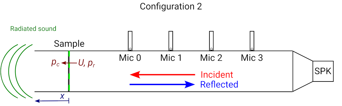
Impedance tube configured with a duct with open end behind the sample.

If we change from configuration 1 to 2, quite some things happen to the system. For example at low frequencies, it will become much harder to generate a high acoustic pressure on the open end side ($p_c$) of the sample, as all air pressure will leak away through sound radiation.

Why is input impedance important?

This is important for determining the right measurement method and getting a high accuracy. We will explain further.

Suppose the sample has a very low series impedance. In that case the input impedance will be completely determined by the boundary condition behind the system (open end vs closed end or others). The low frequency limit can typically be used to indicate what is happening:

• Configuration 1 gives an input impedance that grows indefinitely when we decrease the frequency to 0.
• Configuration 2 gives an input impedance of 0 when we decrease the frequency to 0.

The way we measure the sample series impedance is by computing the input impedance in two configurations. We keep the boundary condition on the left side of the sample the same. First we perform a reference measurement, where only the input impedance is measured without sample. Then we perform the measurement with sample. By determining the input impedance again, the series impedance can be determined by subtracting the input impedance with sample from the case without sample.

This procedure only gives sensible results, when the two impedances differ significantly. Otherwise we are just measuring noise. Thus, the accuracy with which we can determine the series impedance of the sample depends on the accuracy with which we can measure the input impedance.

Impedance tubes have limitations on this, as it is typically difficult to accurately measure high standing wave ratios, due to the small phase differences that it introduces. In the configurations shown above, it is only possible to measure input impedance up to 10 to 50 times the magnitude of the characteristic acoustic impedance in the tube.

If the sample series impedance is such high, the configurations above basically cannot make a difference between a "hard wall" and a sample anymore. This happens for small samples w.r.t. to the tube diameter, often combined with high series impedance samples.

5 microphones

In case the default measurement method is unable to measure the input impedance accurately enough, one can switch to a configuration as follows:

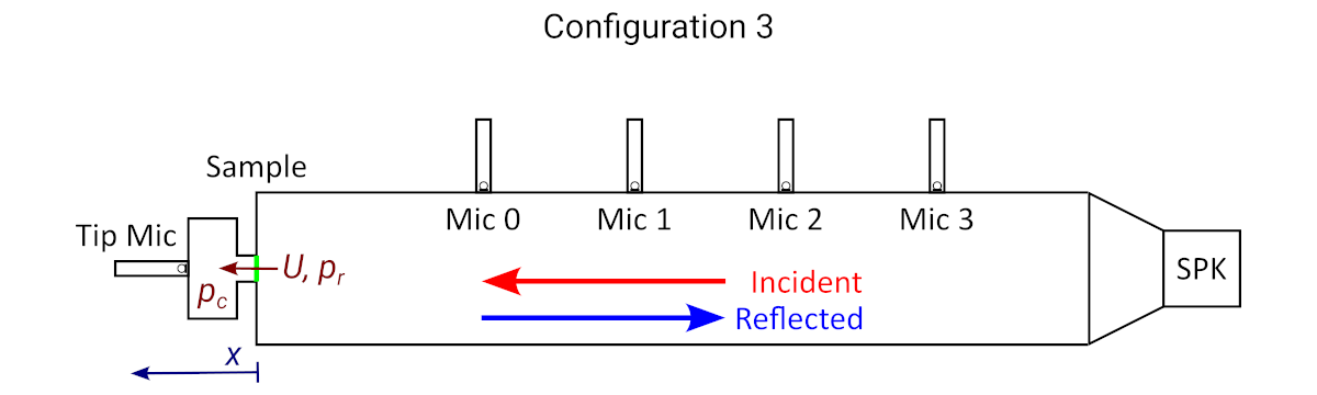
Impedance tube configured with a duct with open end behind the sample.

The 5^th microphone captures the acoustic signal on the other side of the sample, which we call the tip microphone. Using the tip microphone, the volume flow through the sample can be obtained. For example for low frequencies, we know that the tip microphone signal is proportional to the $U/(i\omega)$, i.e. the amount of air that is displaced through the sample. Indeed, a model is required for the cavity behind the sample.

At ASCEE, we have done careful analysis for the size of such a cavity. When we make the cavity too small, this results in:

• Hardly any volume flow through the sample, resulting in the problem that we are interested in the difference between two large numbers.
• Uncertainties due to viscothermal losses in the cavity. For example the compression / expansion will become more isothermal, instead of adiabatic.

On the other hand, making the cavity too large results in:

• A too small signal at the tip microphone, resulting in the measurement of noise.
• at high frequencies, we will have wave effects in the cavity, that require a more complicated cavity model. This is accompanied by extra uncertainty.

All by all, we conclude that this cavity size is a careful consideration, that has to take into account all aspects of the system, and the samples to be measured.

Takeaways

• Series impedance is an actual material property
• Input impedance is important for determining the measurement range and system configuration

In my next post, we will dive into the different normalization options that are in use. Learn more on determining the right measurement configuration for µZ measurements.