What is smoothing? Part 1

October 15, 2025

Introduction

Sometimes a graph is difficult to read. It has lots of unnecessary detail or it fluctuates so much that it becomes uncertain where the line exactly is. Check out the figure below. We are an acoustics company, so we like data in the frequency domain. The blue line is terrible, right? Try to read the value at 6 kHz, good luck with that. Now compare to the orange line, which is much easier to interpret.

We did something. We added 'smoothing'. It makes things smooth.

But what is smoothing? What peculiarities come into play when you actually try to implement it? Let's dive in together.

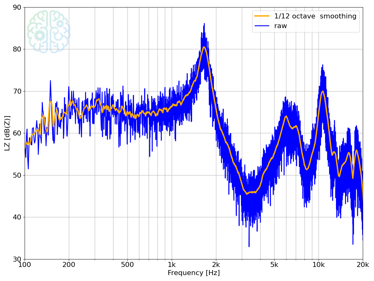
Auto power spectrum of an acoustic measurement, with and without smoothing

Definition

Before we dive into the details, here is a simple definition:

In a smoothed graph, each point is the weighted average of several points around it.

This is best explained with an example.

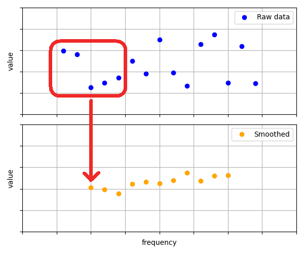
Example

The figure above shows raw and smoothed data. A red window selects five raw points. These are averaged to form a smooth, orange data point. Move the window one point to the right and repeat. As you can see, smoothing is a moving average filter in essence. It has various upgrades that we discuss in the next paragraphs.

Challenge 1: fractional octave smoothing

People tend to plot frequency domain data on a logarithmic frequency scale. Along the frequency axis, each pixel corresponds to a certain number of octaves or fraction of an octave. It matches better with how we hear. The smoothing should accomodate this fact and — optically — add the same amount of 'smoothness' at both the low and high ends of the spectrum. This means that the smoothing width, the width of the window, should be expressed in octaves. It is common to use fractional octaves, like 1/24th octave.

The raw data points, however, are usually the result of a Fast Fourier Transform and therefore have a linear frequency spacing. Then one octave, at a high frequency, covers more data points than an octave at a low frequency. If we view smoothing as a moving average filter, the window does not have a fixed width (expressed in number of points) and has to be updated for each frequency. This can make the calculation computationally expensive.

The logarithmic frequency scale has a second implication. Considering that the window has to look symmetric, the distance between each edge and the center is also expressed in octaves. On a linear frequency scale, the center would not be in the center! The upper half of the window contains more data points than the lower half. The data points should be weighted to avoid a bias towards the upper half.

As a sidenote: the smoothing width does not always encompass an integer number of points. We can simply choose to include points that fully lie within the window, to make it integer. Therefore the actual smoothing width is slightly off from the fractional octave that we want. As long as the window is much wider than the interval between data points, this is not a problem. This does not hold at low frequencies.

Challenge 2: edges

Smoothing one data point requires data from the points around it. But what do you do if that data does not exist? Suppose the sample rate is 48 kHz, making the Nyquist frequency 24 kHz. To smooth the data point at 24 kHz with a 1/6th octave width, we need data from 22.7 ... 25.4 kHz. Between 22.7 ... 24 kHz the data is available but at 24 ... 25.4 kHz it is missing. Uh oh!

There are three options to handle this case:

1. Do not try to calculate a smoothed value.
2. Ignore that data is missing and compute the average of what is available.
3. Symmetrically decrease the smoothing width as you approach the Nyquist frequency.

There is no right or wrong. All methods have their advantages. The first does not compromise on the smoothing quality but obviously does not plot all data. It is the method used in the paragraph Definition. The second retains smoothness all the way up to the Nyquist frequency, but tends to diverge from the raw data if the data slopes up or down. The third method retains the output point centered in its window and therefore handles data with a slope better, but gradually loses its smoothing capability. You can see the effect in the following figure. Towards 24 kHz, the smoothed graph becomes less and less smooth, starting at 22.7 kHz. It is the solution we chose for ACME.

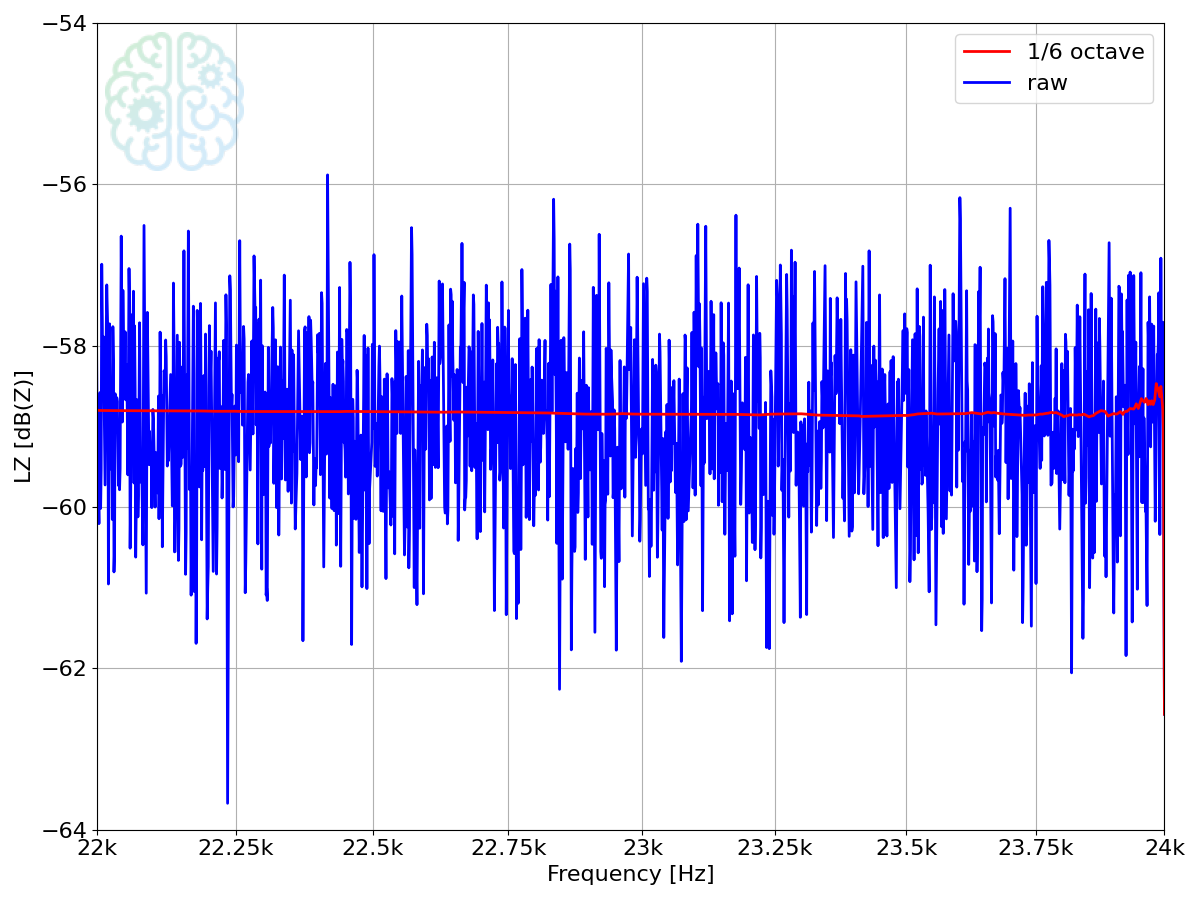
Edge effect at the upper end of the frequency range, smoothed at 1/6th octave

In case you are wondering what happens at the lower end of the frequency range: it is not a problem if we stick to fractional octave smoothing. An FFT outputs data all the way down to "0 Hz", while the smoothing window will never extend to negative frequencies. We still get bad smoothing, but that has a completely different reason: an octave does not contain many points at a low frequency. The smoothing window shrinks down to just a few data points here, perhaps only one.

Challenge 3: make it look good

Aesthetics also count. Smoothed graphs find their way into data sheets and marketing material. So smoothing not only has to make a graph more legible, it also has to look pretty.

Something that can look off with the wrong kind of smoothing, is when the raw data graph has a narrow peak. It can be due to a high Q resonance or a tonal signal. Let us try two kinds of smoothing. Which one do you think looks better?

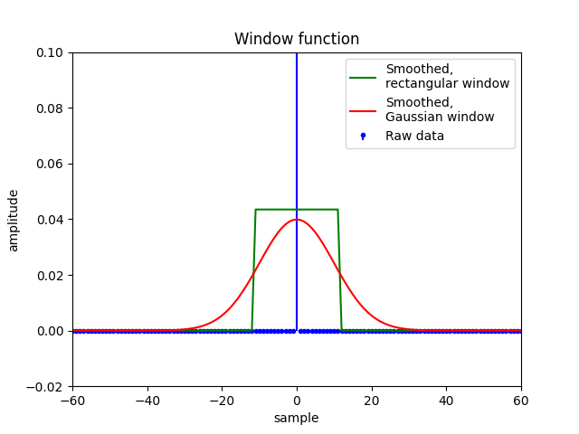
Effect of window function, linear frequency scale. On x=0, the raw data has a value of 1.

Personally, I really like the version with the Gaussian window. The raw data points are not simply averaged, but weighted with a bias on the center. The weight gradually drops towards the edges of the smoothing width. We can do this by multiplying points within the smoothing width with a window function, before averaging them. In this example, it is a Gaussian function.

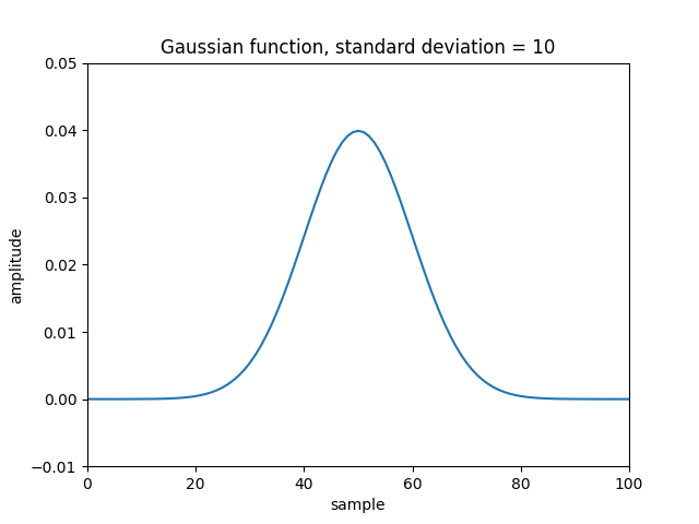
Gaussian function

Because the Gaussian window function is biased to the center, the window has been widened to still add the same amount of smoothness. The function is scaled to have an integral of one.

Wrapping up

We have seen that smoothing can be rough to implement. The number of data points within the smoothing width is constantly changing, points are missing and we need to multiply with a window function to make it look good. If you think these are the only challenges involved with a smoothing implementation, brace yourself for part 2.