What is smoothing? Part 2

November 05, 2025

Introduction

In part 1 of this series, we have seen that spectral smoothing has all sorts of details to pay attention to. The number of data points within the smoothing width is constantly changing, points are missing and we need to multiply with a window function to make it look good. In this part, we continue with aspects that affect the quantitative analysis.

FFT bins

We start by taking a step back to see what data we are working on. This can be for example an auto power spectrum, or a frequency response function. In all cases, they are in the frequency domain. For the spectral smoothing that we discuss here, we only consider the magnitude.

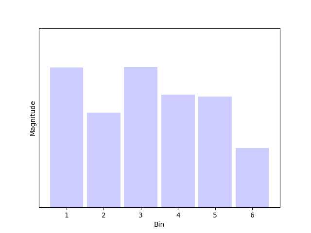
Such data typically are the result of a Fast Fourier Transform (FFT). Each spectral component is assigned to a discrete frequency bin, as shown in the figure below:

Illustration of FFT bins

What's important, is that the bins are.. bins. They are not single frequencies, but cover a certain range. The bin width $\Delta f_\mathrm{bin}$ is related to the FFT length in samples $\mathrm{N_FFT}$ and sample rate $f_s$:

$$\Delta f_\mathrm{bin} = \frac{f_s}{\mathrm{N_{FFT}}} \qquad \mathrm{in\ Hz}$$

From the point of view of the FFT, there are no frequencies other than those of the bins. Please note that we assume that segmented FFT is used: the Fourier transform operates on multiple short sections of the signal and the power result are summed of averaged. An advantage is that it reduces memory consumption and speeds up calculations. A tradeoff is that short FFT length decreases the frequency resolution and therefore increases the bin width.

Challenge 4: absolute peak height

As discussed in part 1, smoothing is like a moving average filter. It mows down narrow peaks and spreads them across a wider range. If the peak width is limited to a single bin (the algorithm has no way to tell if it is even narrower), the power within that bin is calculated as the product of its height and width, after which it is redistributed across the smoothing width. Sounds reasonable, right?

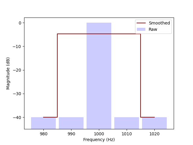
Say, the original time domain signal is a 1000 Hz sine wave with amplitude 1. In the frequency domain, the spectrum magnitude is zero (drawn as -40 dB, corresponding to some fictional noise floor), except for one bin at which it is 0 dB.

If the bin width is 10 Hz and the smoothing width 30 Hz wide, there are 3 bins to distribute the power across and the peak height decreases to -5 dB. So far so good, smoothing was supposed to make peaks lower and wider, which it did.

1 kHz pure tone captured in a wide bin and the smoothed result

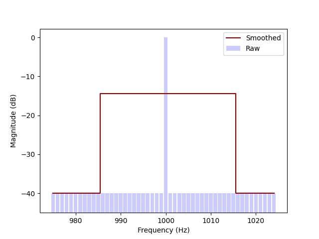
We start over but pick longer FFT length, corresponding to a bin width of 1 Hz. The smoothing width is still 30 Hz wide. After smoothing, the peak is just as wide, but now reaches to -15 dB, as the power had to be divided across ten times as many bins. This cannot be right? Apparently, the result depends on the FFT length — not a desirable property!

1 kHz pure tone captured in a narrow bin and the smoothed result

We got into a subtlety here. Strictly speaking, smoothing should not be applied to a power spectrum. That is because the bin width depends on the FFT length, while the peak height does not. Smoothing should only be applied to a power spectral density, which is similar to a spectrum but scaled to compensate for the FFT length.

For this example, the magnitude of the power spectral density after smoothing is independent of bin width. In this example of a pure tone, the spectral density would go to infinity if the bin width approaches zero.

In practice, we can get away with this for qualitative analyses. Just remember that smoothing makes the absolute peak height meaningless, as the power is spread over multiple frequency bins.

Challenge 5: retaining power

Statistics on smoothed data should be approximately the same as on raw data. It would be weird if a smoothing operation changed the total power. In order to keep the power the same, each raw data point should be counted exactly once in the smoothed data.

Consider smoothing to be a multiplication of the raw data vector with a smoothing matrix:

$$ \mathbf{v}_{\mathrm{smoothed}} = \mathbf{M} \cdot \mathbf{v}_{\mathrm{raw}}$$

If the columns of the matrix $\mathbf{M}$ are normalized to 1, then the cumulative contribution of each raw data point is one. The normalization, however, has two serious drawbacks:

1. The easiest way to implement normalization across the columns, is to first build the whole matrix. That would result in serious memory consumption if the $\mathrm{N_FFT}$ is large: with a not unrealistic $\mathrm{N_FFT}$=48k, the matrix would have (48k)$^2$ = 2.3 billion elements. Assuming the matrix is not sparse and all elements are 64 bit floats, it would take 18 GB of memory.

2. In part 1 - edge effects, we have seen different options on how to handle missing data. With normalization across the columns, the smoothing algorithm implicitly chooses for something similar to option 2: the points near the edge are progressively counted more heavily, to compensate for them not being used to smooth frequencies beyond the nyquist frequency.

A more feasible option is to try to retain power only at the bulk of the frequency range and not at the edges. This can be implemented by normalizing the smoothing window such that its integral is 1. There is no need to build the matrix at once. We can simply calculate one row, multiply it by the raw data vector and store the resulting point in the smoothed data vector. This is the method that ACME uses.

Challenge 6: phase

Up to now, we have only considered the magnitude and assumed to smooth power, which does not have a phase. However, in general data in the frequency domain is not complete without its phase data. Can a frequency response function be smoothed as well? There is not a clear method. How would you average two neighbouring points in the frequency domain, one with magnitude 1 and phase 0, the other with magnitude 1 and phase π? Does their magnitude average to 0 or 1? Does the phase average to 0.5 π, 1.5 π or is it undefined? There is no way to unambiguously smooth it.

Another factor is that the presence of phase data would make it possible to apply an inverse FFT (IFFT), to convert the result to the time domain. As you have seen by now, there is not a single true way to smooth: all kinds of choices have to be made. It is possible that the result of an IFFT contains ringing or is non-zero for negative time. Then the result would be somewhat meaningless. We therefore say for now: smoothing phase data is not allowed.

Wrapping up

Care should be taken when using smoothing, if a qualitative analysis is to be performed afterwards. The operation can change the absolute peak height of pure tones, in a way which depends on the FFT length. It does not necessarily retain power and phase data is either lost or ambiguous. Take your time to check whether it applies to your analysis. Slow is smooth and smooth is fast!