
A customer wanted to understand how sound propagates in specific wave patterns. Normally, we solve this in COMSOL using the Westervelt equation. But when the distances become large and the wavelength is small, the computation time and memory requirements often get completely out of hand.
At that point, we need to adopt a smarter approach to arrive at a solution within a reasonable computation time. For nonlinear waves, it turns out that you can calculate the change in the waveform while tracking the wave from its source. We call this coordinate system the delayed time frame, expressed as:
\[t' = t - \frac{z}{c_0}\]Here, \(t\) is the actual time, \(z\) is the perpendicular distance from the source, and \(c_0\) is the speed of sound. By using this time-delayed frame of reference, we do not need to solve the wave equation over the entire spatial domain. We simply track how the waveform changes over the distance traveled. The disadvantage of this transformation is that we can only solve for one propagating wave at a time.
The mathematical model that describes a nonlinear wave in the time-delayed frame is called the KZK equation [1]. It would go beyond the scope of this case study to discuss the model in detail, but essentially, it calculates the change in the waveform based on three effects:
– Nonlinear wave steepening
– Viscous and thermal damping
– Geometric dispersion
In linear theory, two acoustic waves travel right through each other without any interaction. In nonlinear theory, this is not the case. The KZK model can therefore only calculate the behavior of a single propagating wave.
We have built our own modern KZK solver in Rust. Thanks to Rust’s concurrency model, this software performs highly parallel computations. This is possible because the three physical effects can be added together, allowing us to compute them independently of one another.
Below is a screenshot of a simulation in progress:
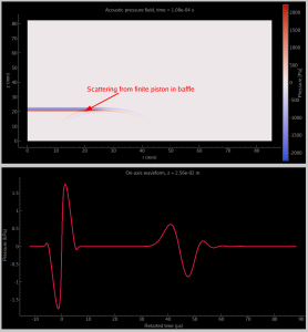
The calculated example concerns the classic radiation from a piston into an infinite screen, but at a high amplitude. The effects of this high amplitude lead to wave stiffening, which ultimately results in a sawtooth-shaped wave:
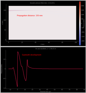
The results already show shock wave formation at a distance of 150 millimeters from the source. This occurs only at very high amplitudes. In this example, the pressure amplitude is approximately 1 kPa, which corresponds to 148 dB SPL. These are sound levels comparable to the firing of firearms. A video of the simulation can be found here.
This software was developed to investigate various acoustic effects associated with finite-amplitude waves. One example is intermodulation distortion. This can be used to generate audible sound through the interaction of two ultrasonic frequencies. We have previously presented this mechanism in detail; you can find that explanation here.
Another notable effect of high-amplitude sound is acoustic radiation pressure. This is a time-averaged force generated by the sound source. This principle enables new techniques for manipulating small objects without physical contact, such as with acoustic tweezers.
At ASCEE, we have the in-house simulation software to perform numerical analyses of these mechanisms. We can immediately provide you with the correct parameters for, for example, sizing the required transducer or determining the optimal frequency. In addition to nonlinear waves in free space, we have also developed computational software for high-amplitude sound waves in narrow tubes. See, for example, our publication on the numerical simulation of nonlinear thermoviscous acoustic wave propagation.
What is your next step in simulating nonlinear acoustics?
[1] Lee, Y.-S., and Hamilton, M. F. (1995). “Time-domain modeling of pulsed finite-amplitude sound beams,” The Journal of the Acoustical Society of America 97, 906–917.